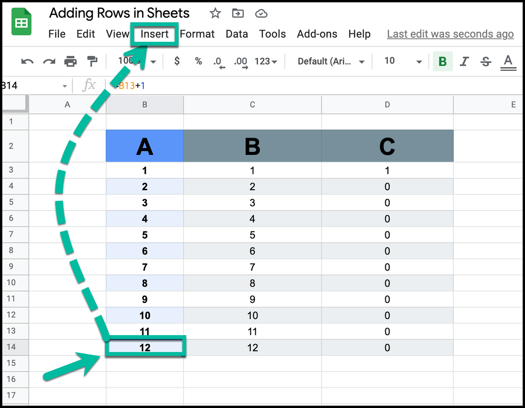
 Integrate Zoho Data Professional with Google Sheets to automatically insert rows in Google Sheets upon a new entry. Configure the spreadsheet extension to automatically insert rows in Google Sheets upon a new entry when a relevant new record is added in Zoho Data Professional. Users may also manually import data from Zoho Data Professional into Google Sheets, again on-demand, to create actionable data. The ability to do this may be used for creating reports, for creating reminders, or for tracking multiple lists. In this guide, we will demonstrate the entire process, step-by-step, using examples that include two users who have each imported data from different applications: a company representative and a customer. After clicking the + sign button next to the word imported, an empty Worksheet is displayed. Click on the cell for a name, then type a unique name for the account and the page in the Spreadsheet. In this example, the page refers to the webpage for a hypothetical company and the company representative has entered the URL for the website at the end of the URL. Open a new workbook in Excel, create a new data source, and then import the required data from Google into the worksheet. To import the data, select the appropriate form, fill in the required information, and then click the "Create" button. Google Sheets will ask if the user wants to import multiple rows and click "Go". A wizard will now appear and will prompt the user to select a destination for the imported data. Once the destination is selected, Excel will display the location where the imported data will be located - in this example, the workbook will be linked to the Google sheet in the corresponding directory. If you would love to understand how to insert rows in google sheets, make sure you click this link. To make it easier to manage and use your Google records, it is helpful to have an automated system in place that can import and manage the various data sources. This is where the third party software comes in to play! With these software programs, you can automatically insert rows in Google sheets in a matter of minutes. Some of the software programs are available for free and some of them are a bit more expensive. The free software programs are usually very basic and do not have the advanced features that the more costly programs have, but they are still well worth looking at and trying out. One of the most popular software programs that is available for importing and managing information from Google is the Microsoft Get Response. It is also free to download and use. This software allows the user to easily create an automatic insertion of rows in Google sheets and then update and manage the data source using the built-in Microsoft Outlook Express client. This makes it very easy to keep track of your employees' contact information, job history, company details, and much more all in one place, which is exactly what you need if you want to integrate crm with your Google sheets. See this site to learn how to insert rows in google sheets at this instant. If you do not want to lock your entire google spreadsheet, there is another option available. All you have to do is create a table, label it, and then copy and paste the information you want to include into the table. When you do this, the Google sheet will be locked and you can not change any of the cells once the data has been inserted into them. This is the easiest and least intrusive way to integrate crm with your sheets because none of the data is locked into the Google spreadsheet. The only thing you have to do is select the appropriate table, label it, and copy and paste the information. This is an easy way to have an automatic insert row in your Google sheet! For you to get more enlightened about this subject, see this post: https://en.wikipedia.org/wiki/Google_Sheets.
0 Comments
7/21/2021 0 Comments Find Duplicates in Google Sheets Using Dynamic Formula or a dynamic Pivot Table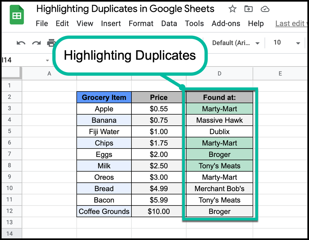 Open the spreadsheet that you wish to analyze in Google Sheets. Ensure that the spreadsheet has all data arranged by rows and each row has a header. Highlight the column where you wish to search through and enter the query you wish to perform. Type the query into the text box. If there is a matching unique function, click the Search button. In Excel, you may find the matching query by clicking the Query / Find in the drop down menu. In Excel, you may find the matching query by clicking on Formula / Other and then click on AutoFit. Then click OK. Open a new file in MS Excel and then highlight duplicates in Google Sheets by highlighting the cells you wish to search. Right click the highlighted cells and choose Insert and copy the contents of the second cell onto your worksheet. Open conditional formatting and change the values to False and true. In Excel, you will also find a similar option. Select Home tab and then click on Format From. Then type the entire column into the text box. Click OK. Open another file in MS Excel and highlight the entire column again. Click here to learn how to find duplicates in google sheets. The above two ways may be used to find duplicate data in Google Sheets but the same can be achieved in a much easier way. This method uses a function that calculates the duplicates of any value in a column. To do this, type the value you are calculating the duplicate of in the second cell and then press the calculated columns button. This will display all the values that are found in the first cell marked as Duplicates. If you only need the first cell, choose the drop-down menu and select All to Display and the data will be displayed in the format specified. Another easy way to find duplicates in Google sheets is by using the Dynamic Formula option. This is available under the Tools menu and is a known value that is a combination of one or more dynamic functions. By using the drop-down menu, select Formula and then type the entire column into the text box. Hit on the OK button to close the formula. To find the exact values that you need in a range of cells, use the Open Conditional Formatting option and click the button for the range that you want to analyze. There is now an additional drop-down menu for the columns that you wish to analyze and this will give you the option of typing a range of values into the text box. You can choose the exact columns that you need in the cell ranges that are already selected. The drop-down list will show all the columns that match the criteria you have given and will display the value in the cell. If you have entered an incorrect number of columns the results will be wrong. If you would like to know how to find duplicates in google sheets, see this webpage now! Using the above methods will eliminate duplicates in Google sheets by calculating their differences before they are grouped together. This will ensure that the results shown in the report are the most accurate possible. However, there is a better way to do this task. The Open Data Taskforce (ODTF) provides a very flexible and easy to use analytical tool that can perform calculations automatically. You can also save all your calculations to a CSV file and easily analyze the data. Click this link: https://en.wikipedia.org/wiki/Google_Docs_Editors to get more enlightened about the topic discussed in the article above. 7/21/2021 0 Comments How to Subtract In Google Sheets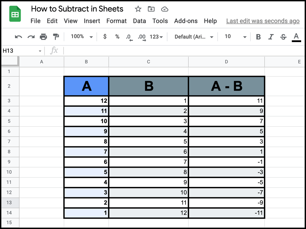 If you are trying to understand how to subtract in Google Sheets, then you should start by opening a new document. On the File menu, click "sheets" and on the "Add" drop down menu, select "Google Sheets". In the Add a New Sheet dialog box, enter the following formula into cell A2: =Sqrt(A2-1) If the above formula is incorrect or if you cannot provide a valid range for the subtracted value, then Google will display an error message. To fix this problem, supply a range in the Excel spreadsheet that identifies the invalid range. Open Microsoft Excel to find out how to subtract in Google Sheets by using the minus function. Click the Down arrow button on the top right corner of the worksheet. In the drop down menu, click the drop down menu for "Subtract". In the Select Value dialogue box, click the minus sign and type the number to be subtracted. If you would like to know how to subtract in google sheets, click here. Using the Google Sheets custom drop down menu, select "API Reference" and in the drop down menu, click the link that appears next to the request URL. In the Request URL text box, type the following formula into cell A2: =Sqrt(A2-1) This formula is an ordinary minus operator. When the user enters a negative number into the Google sheet range, a subtraction is performed on the first number that is entered. This means that the second number is subtracted and so on until all numbers are calculated. Once this operation is completed, the spreadsheet is ready to be used. There are two ways to perform the Google sheet subtractions. The first method is to use the drop-down menus to select "Subtract" and the second way is to use the formulas cell values in cells A1 to C. To find the formula used to perform the Google sheet subtraction, go to the formulas section of the Google sheet where you can access them. For this example, we will start with the first cell in the spreadsheet, which is the Home input. Right click on this cell, go down to "Cell Formatting" and then click on "igraphal". This will open a new page where you can find instructions to subtract numbers directly. See this webpage to find out how to subtract in google sheets now! You can find instructions for all the different methods for performing Google subtraction in Google sheets by clicking on the links below. After you have learned how to subtract numbers directly in Google sheets, you will probably want to learn how to perform other types of mathematical calculations. You may even decide to make your own mathematical expressions on your spreadsheets. It is a very fun and exciting hobby, one that I'm sure you will continue to enjoy throughout your life! To understand more about this topic, it is wise to check out this post: https://en.wikipedia.org/wiki/Spreadsheet. |
